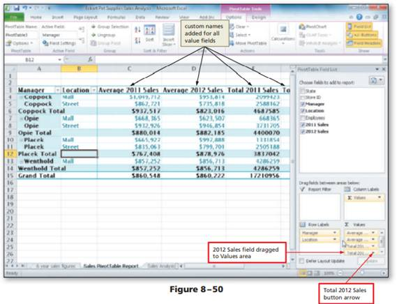
Click the OK button (Value Field Settings dialog box) to apply the custom name to the 2011 Sales fi eld.
• Drag the 2012 Sales fi eld to the Values area to add the fi eld to column F of the PivotTable.
• Click the Sum of 2012 Sales button, and then click Value Field Settings to display the Value Field Settings dialog box.
• Enter Total 2012 Sales in the Custom Name text box to rename the value fi eld.
• Click the OK button (Value Field Settings dialog box) to apply the custom name.
• Use the Value Field Settings dialog box to customize the names as shown in cells C3 and D3 (Figure 8 – 50).
The Correct Answer and Explanation is :
Correct Answer:
- Apply the custom name to the 2011 Sales field:
- In the Value Field Settings dialog box, after entering the desired custom name, click the OK button. This applies the name change to the 2011 Sales field in the PivotTable.
- Add the 2012 Sales field:
- Drag the 2012 Sales field to the Values area. This will add the field to column F of the PivotTable.
- Rename the 2012 Sales field:
- Click the Sum of 2012 Sales button in the PivotTable, then select Value Field Settings.
- In the Custom Name text box, type Total 2012 Sales.
- Click the OK button to apply the new name.
- Customize names in cells C3 and D3:
- Use the Value Field Settings dialog box for each field to update the custom names displayed in the PivotTable, ensuring they match the names shown in Figure 8-50.
Explanation (300 Words):
The Value Field Settings dialog box in Excel allows users to modify how data is summarized, displayed, and named in a PivotTable. These settings are essential for improving the readability and usability of PivotTables, especially when dealing with multiple fields or large datasets.
In this example, the task involves customizing field names for better clarity. First, renaming the 2011 Sales field is done by accessing the Value Field Settings dialog box and entering a descriptive name (e.g., Total 2011 Sales) in the Custom Name text box. Clicking the OK button confirms the change, and the new name is displayed in the PivotTable.
Next, the 2012 Sales field is dragged into the Values area, automatically placing its data in column F. By default, Excel names the field based on its data aggregation method (e.g., Sum of 2012 Sales). To make this label more meaningful, the Value Field Settings dialog box is used again. The field is renamed Total 2012 Sales, reflecting its purpose more clearly.
Finally, the names for other fields (e.g., in cells C3 and D3) are customized using the same process, ensuring consistency with the labels shown in Figure 8-50. These steps improve the PivotTable’s clarity, making it easier to analyze and present the data.
Such techniques are critical for professionals who need to prepare data reports that are intuitive and tailored for specific audiences. By leveraging these features, users enhance both the functionality and appearance of their PivotTables.