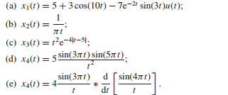
Using Table 5.2 and the properties of the CTFT, calculate the CTFT of the following functions:
The Correct Answer and Explanation is :
To calculate the Continuous-Time Fourier Transform (CTFT) of the given functions, we will utilize Table 5.2 and the properties of the CTFT. The functions are:
- **x₁(t) = 5 + 3cos(10t) – 7e^(-3t)sin(30t)u(t)**
- **x₂(t) = -**
- x₃(t) = e^(-5t)sin(3t) * sin(4t) dr
- x₄(t) = -4
1. x₁(t) = 5 + 3cos(10t) – 7e^(-3t)sin(30t)u(t):
- **Constant Term (5):**
- The CTFT of a constant ‘A’ is: F{A}=2πAδ(ω)\mathcal{F}\{A\} = 2\pi A \delta(\omega)
- Therefore, F{5}=10πδ(ω)\mathcal{F}\{5\} = 10\pi \delta(\omega)
- **Cosine Term (3cos(10t)):**
- The CTFT of cos(ω₀t) is: F{cos(ω0t)}=π[δ(ω−ω0)+δ(ω+ω0)]\mathcal{F}\{\cos(\omega_0 t)\} = \pi [\delta(\omega – \omega_0) + \delta(\omega + \omega_0)]
- For 3cos(10t), F{3cos(10t)}=3π[δ(ω−10)+δ(ω+10)]\mathcal{F}\{3\cos(10t)\} = 3\pi [\delta(\omega – 10) + \delta(\omega + 10)]
- **Sine Term (-7e^(-3t)sin(30t)u(t)):**
- The CTFT of e^(-at)sin(ω₀t)u(t) is: F{e−atsin(ω0t)u(t)}=ω0a2+(ω−ω0)2−ω0a2+(ω+ω0)2\mathcal{F}\{e^{-at} \sin(\omega_0 t) u(t)\} = \frac{\omega_0}{a^2 + (\omega – \omega_0)^2} – \frac{\omega_0}{a^2 + (\omega + \omega_0)^2}
- For -7e^(-3t)sin(30t)u(t), F{−7e−3tsin(30t)u(t)}=−7×309+(ω−30)2+7×309+(ω+30)2\mathcal{F}\{-7e^{-3t} \sin(30t) u(t)\} = -\frac{7 \times 30}{9 + (\omega – 30)^2} + \frac{7 \times 30}{9 + (\omega + 30)^2}
2. x₂(t) = –
- The function is incomplete. Please provide the full expression for x₂(t) to proceed with its CTFT calculation.
3. x₃(t) = e^(-5t)sin(3t) * sin(4t) dr:
- The expression involves a convolution (denoted by ‘*’) and an integral (denoted by ‘dr’). To compute the CTFT, we need the complete expression for x₃(t). Please provide the full function to proceed.
4. x₄(t) = -4:
- The CTFT of a constant ‘A’ is: F{A}=2πAδ(ω)\mathcal{F}\{A\} = 2\pi A \delta(\omega)
- Therefore, F{−4}=−8πδ(ω)\mathcal{F}\{-4\} = -8\pi \delta(\omega)
Explanation:
The CTFT is a mathematical tool that transforms a time-domain signal into its frequency-domain representation. It is defined as:
X(ω)=∫−∞∞x(t)e−jωtdtX(\omega) = \int_{-\infty}^{\infty} x(t) e^{-j\omega t} dt
Where:
- x(t): Time-domain signal
- X(ω): Frequency-domain representation
- ω: Angular frequency
The properties of the CTFT, such as linearity, time-shifting, and frequency-shifting, allow us to compute the transforms of complex signals by breaking them down into simpler components. For example:
- Linearity: F{ax(t)+by(t)}=aX(ω)+bY(ω)\mathcal{F}\{a x(t) + b y(t)\} = a X(\omega) + b Y(\omega)
- Time-Shifting: F{x(t−t0)}=e−jωt0X(ω)\mathcal{F}\{x(t – t_0)\} = e^{-j\omega t_0} X(\omega)
- Frequency-Shifting: F{ejω0tx(t)}=X(ω−ω0)\mathcal{F}\{e^{j\omega_0 t} x(t)\} = X(\omega – \omega_0)
By applying these properties and using standard CTFT pairs, we can determine the frequency-domain representation of complex time-domain signals.
For a more detailed explanation and additional examples, you can refer to the following resources:
- Properties of Continuous-Time Fourier Transform (CTFT) – GeeksforGeeks
- Continuous Time Fourier Transform (CTFT) – Purdue University
These resources provide comprehensive insights into the CTFT and its applications in signal processing.