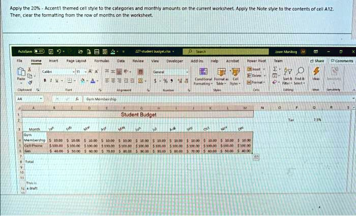
Apply the 20% – Accent1 themed cell style to the categories and monthly amounts on the current worksheet. Apply the Note style to the contents of cell A12. Then, clear the formatting from the row of months on the worksheet.
The Correct Answer and Explanation is:
To complete the request, you will perform three distinct formatting actions on the Excel worksheet.
First, apply the “20% – Accent1” cell style. To do this, you must select the range of cells containing the expense categories and their corresponding monthly values. This specific range is A4:M6. After selecting these cells, navigate to the Home tab on the ribbon. In the Styles group, click the Cell Styles button to open the gallery of available styles. Under the “Themed Cell Styles” section, locate and click on 20% – Accent1. This will apply a light orange fill and other formatting to the selected data, visually grouping the budget’s core information.
Second, apply the “Note” style to the text in cell A12. Begin by selecting cell A12, which contains the text “a draft”. Go back to the Home tab and click the Cell Styles button again. In the style gallery, find and select the Note style. This action will typically change the font style and add a light background color, making the text in cell A12 stand out as an annotation or comment separate from the primary budget data.
Third, you need to clear the formatting from the row of months. The months are located in the range B3:M3. Select this range of cells. With the cells selected, go to the Home tab. In the Editing group on the far right, click the Clear command, which is represented by an eraser icon. A dropdown menu will appear. From this menu, choose Clear Formats. This will remove the background color, font styling, and any borders from the month headers, resetting them to the worksheet’s default cell format while leaving the text (“Jan”, “Feb”, etc.) intact.