Gradient and Hessian of log-likelihood for multinomial logistic regression
The gradient and Hessian of the log-likelihood function for multinomial logistic regression are essential for optimization in parameter estimation. Here’s how they are derived and expressed:
Log-Likelihood Function
For nn data points and KK classes, let:
- xi\mathbf{x}_i be the feature vector for observation ii,
- βk\mathbf{\beta}_k be the coefficient vector for class kk,
- yiy_i be the true class label of observation ii,
- pikp_{ik} be the predicted probability for observation ii and class kk.
The probability of yiy_i given xi\mathbf{x}_i is: p(yi=k∣xi)=exp(βk⊤xi)∑j=1Kexp(βj⊤xi).p(y_i = k | \mathbf{x}_i) = \frac{\exp(\mathbf{\beta}_k^\top \mathbf{x}_i)}{\sum_{j=1}^K \exp(\mathbf{\beta}_j^\top \mathbf{x}_i)}.
The log-likelihood is: ℓ(β)=∑i=1n∑k=1K1(yi=k)logpik.\ell(\mathbf{\beta}) = \sum_{i=1}^n \sum_{k=1}^K \mathbf{1}(y_i = k) \log p_{ik}.
Here, 1(yi=k)\mathbf{1}(y_i = k) is an indicator function equal to 1 if yi=ky_i = k, and 0 otherwise.
Gradient of the Log-Likelihood
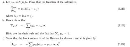
Define πik=pik\pi_{ik} = p_{ik}, the predicted probability. The gradient with respect to βm\mathbf{\beta}_m is: ∂ℓ∂βm=∑i=1nxi(1(yi=m)−πim).\frac{\partial \ell}{\partial \mathbf{\beta}_m} = \sum_{i=1}^n \mathbf{x}_i \left( \mathbf{1}(y_i = m) – \pi_{im} \right).
Hessian of the Log-Likelihood
The Hessian matrix HH consists of second derivatives: Hm,j=∂2ℓ∂βm∂βj.H_{m,j} = \frac{\partial^2 \ell}{\partial \mathbf{\beta}_m \partial \mathbf{\beta}_j}.
For a single data point ii: Hm,j(i)=−xixi⊤πim(δmj−πij),H_{m,j}^{(i)} = – \mathbf{x}_i \mathbf{x}_i^\top \pi_{im} (\delta_{mj} – \pi_{ij}),
where δmj\delta_{mj} is the Kronecker delta (1 if m=jm = j, 0 otherwise).
Summing over all data points: Hm,j=∑i=1nHm,j(i).H_{m,j} = \sum_{i=1}^n H_{m,j}^{(i)}.
Summary
- Gradient:
∂ℓ∂βm=∑i=1nxi(1(yi=m)−πim).\frac{\partial \ell}{\partial \mathbf{\beta}_m} = \sum_{i=1}^n \mathbf{x}_i \left( \mathbf{1}(y_i = m) – \pi_{im} \right).
- Hessian:
Hm,j=−∑i=1nxixi⊤πim(δmj−πij).H_{m,j} = – \sum_{i=1}^n \mathbf{x}_i \mathbf{x}_i^\top \pi_{im} (\delta_{mj} – \pi_{ij}).
These expressions are used in optimization algorithms like Newton-Raphson to estimate the model parameters. If you need further assistance or detailed derivations, feel free to ask!