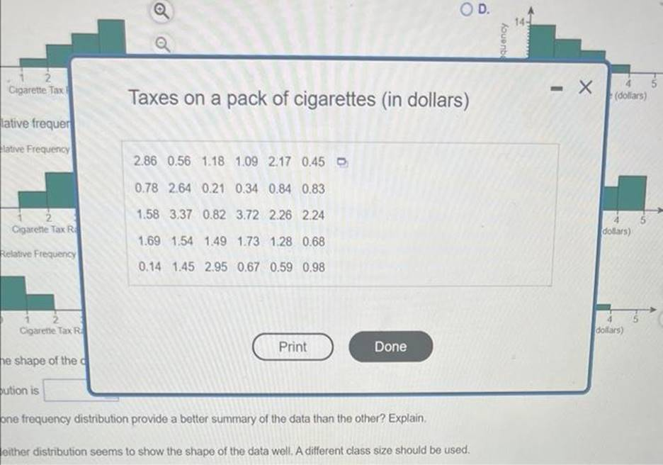
caprete tax Taxes on a pack of cigarettes (in dollars) lative frequer 4ative Frequency Relative Frequency oution is one frequency distribution provide a better summary of the data than the other? Explain. leither distribution seems to show the shape of the data well. A different class size should be used. The accompanying table shows the tax, in dollars, on a pack of cigarettes in 30 randamly selected cities. Complete parts (a) through (g) below. Click the icon to view the table of data. (a) Construct a frequency distribution. Use a first class having a lower class limit of 0 and a class width of 0.50. (Type inteoers or decimals. Do not round.) (b) Construct a relative frequency distribution. Use a first class having a lower class limit of 0 and a class widh of 0.50 iDnient th then davimal nlarse as neadiad I (c) Construct a frequency histogram. Choose the correct graph below. A. C. (d) Construct a relative frequency histogram. Choose the correct graph below. D. A. C. B. D. (f) Repeat parts (a)-(0) using a class width of 1 . Construct a frequoncy distribution. Construct a relative frequency distribution. (Round to two decimal places as needed.) Construct a frequency histogram. Choose the correct frequency histogram beion.
The correct answer and explanation is:
Let’s walk through each step for the problem involving the tax on a pack of cigarettes across 30 randomly selected cities.
Part (a) Frequency Distribution with Class Width of 0.50
We are asked to create a frequency distribution, using a class width of 0.50 and a lower class limit of 0. The steps to complete this are:
- Determine Class Ranges: Start with 0 and add 0.50 to each subsequent class:
- Class 1: 0.00 – 0.50
- Class 2: 0.50 – 1.00
- Class 3: 1.00 – 1.50
- Continue for as many classes as necessary to cover all data points.
- Count the Data in Each Class: Look at each city’s tax data and count how many values fall into each class.
- Frequency Distribution Table: Once you have the counts, fill out the frequency table with the class ranges and their corresponding frequencies.
Part (b) Relative Frequency Distribution
The relative frequency is calculated by dividing the frequency of each class by the total number of observations (in this case, 30).
- Formula for Relative Frequency: Relative Frequency=Frequency of ClassTotal Number of Observations\text{Relative Frequency} = \frac{\text{Frequency of Class}}{\text{Total Number of Observations}} Multiply by 100 if you need percentages.
- Relative Frequency Distribution Table: Create a new table with class ranges and their respective relative frequencies.
Part (c) Frequency Histogram
A frequency histogram is a bar graph where:
- The x-axis represents the class intervals.
- The y-axis represents the frequencies (or counts).
Make sure to:
- Label the axes with class intervals and frequency values.
- Draw bars where the height of each bar corresponds to the frequency for that class.
Part (d) Relative Frequency Histogram
Similar to the frequency histogram, but:
- The y-axis represents relative frequency (or percentages) instead of raw frequencies.
- Bars will reflect relative frequency.
Part (f) New Distribution with Class Width of 1
Repeat the process, but now using a class width of 1 (instead of 0.50). The classes will be:
- Class 1: 0.00 – 1.00
- Class 2: 1.00 – 2.00
- And so on.
Why This Approach Works
The frequency distribution and relative frequency distribution offer a concise summary of the data. A frequency distribution helps us identify how many data points fall into specific ranges, while a relative frequency distribution standardizes the data, allowing for easier comparison across different datasets. The histogram provides a visual representation of the data, allowing for a quick understanding of the distribution shape (e.g., skewed, symmetrical). The relative frequency histogram helps contextualize the data by showing the proportion of each class.
Each distribution type provides different insights into the data, and using the correct class width ensures a clear, interpretable summary.