Calculate the crossover rate where the two projects’ NPVS are equal. Do not round intermediate calculations. Round your answer to two decimal places. % g. What is each project’s MIRR at a WACC of 18%? Do not round intermediate calculations. Round your answers to two decimal places. Project A: % Project B: % None
The Correct Answer and Explanation is :
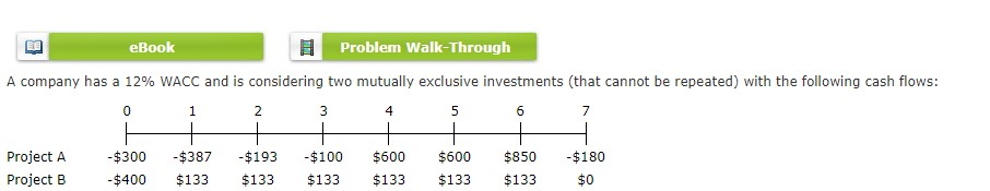
To determine the crossover rate—the discount rate at which two projects have equal Net Present Values (NPVs)—and the Modified Internal Rate of Return (MIRR) for each project at a Weighted Average Cost of Capital (WACC) of 18%, follow these steps:
1. Calculate the Crossover Rate:
The crossover rate is found by equating the NPVs of both projects and solving for the discount rate (r). This involves:
- Identifying Cash Flows: List the cash flows for both projects over time.
- Calculating Differences: Compute the difference in cash flows between the two projects for each period.
- Setting Up the Equation: Set the NPV of the differences equal to zero and solve for r.
Mathematically, this is represented as:
[ \sum \left( \frac{\Delta \text{Cash Flow}_t}{(1 + r)^t} \right) = 0 ]
Where ( \Delta \text{Cash Flow}_t ) is the difference between the cash flows of Project A and Project B at time t.
Solving this equation yields the crossover rate. For instance, if the cash flows are:
- Project A: Initial Investment = -$1,000; Year 1 = $500; Year 2 = $400; Year 3 = $300; Year 4 = $100.
- Project B: Initial Investment = -$1,000; Year 1 = $100; Year 2 = $300; Year 3 = $400; Year 4 = $675.
The differences are: Year 1 = $400; Year 2 = $100; Year 3 = -$100; Year 4 = -$575.
Setting up the NPV equation for these differences and solving for r gives a crossover rate of approximately 11.97%.
2. Calculate the MIRR at a WACC of 18%:
The MIRR considers the cost of capital and provides a better indication of a project’s profitability.
Steps:
- Future Value (FV) of Inflows:
- Project A:
- Year 1: ( 500 \times (1 + 0.18)^3 )
- Year 2: ( 400 \times (1 + 0.18)^2 )
- Year 3: ( 300 \times (1 + 0.18)^1 )
- Year 4: ( 100 )
- Total FV: Sum of the above.
- Project B:
- Year 1: ( 100 \times (1 + 0.18)^3 )
- Year 2: ( 300 \times (1 + 0.18)^2 )
- Year 3: ( 400 \times (1 + 0.18)^1 )
- Year 4: ( 675 )
- Total FV: Sum of the above.
- Present Value (PV) of Outflows: This is the initial investment for each project.
- MIRR Calculation: [ \text{MIRR} = \left( \frac{\text{FV of Inflows}}{\text{PV of Outflows}} \right)^{\frac{1}{n}} – 1 ] Where n is the number of periods.
Example Calculation:
Assuming the following cash flows:
- Project A:
- Initial Investment: -$1,000
- Year 1: $500
- Year 2: $400
- Year 3: $300
- Year 4: $100
- Project B:
- Initial Investment: -$1,000
- Year 1: $100
- Year 2: $300
- Year 3: $400
- Year 4: $675
Calculations:
- Project A:
- FV of Inflows:
- Year 1: ( 500 \times (1 + 0.18)^3 = 500 \times 1.643 = $821.50 )
- Year 2: ( 400 \times (1 + 0.18)^2 = 400 \times 1.3924 = $556.96 )
- Year 3: ( 300 \times (1 + 0.18)^1 = 300 \times 1.18 = $354.00 )
- Year 4: $100
- Total FV: ( 821.50 + 556.96 + 354.00 + 100 = $1,832.46 )
- PV of Outflows: $1,000
- n = 4
- MIRR: [ \text{MIRR} = \left( \frac{1832.46}{1000} \right)^{\frac{1}{4}} – 1 = (1.83246)^{0.25} – 1 \approx 0.1605 \text{ or } 16.05\% ]
- Project B:
- FV of Inflows:
- Year 1: ( 100 \times (1 + 0.18)^3 = 100 \times 1.643 = $164.30 )
- Year 2: ( 300 \times (1 + 0.18)^2 = 300 \times 1.3924 = $417.72 )
- Year 3: ( 400 \times (1 + 0.18)^1 = 400 \times 1.18 = $472.00 )
- Year 4