Consider the arrangement of two point-C charges as shown in the figure. Calculate the total electric field at point a. Calculate the total electric field at point b. Calculate the total electric potential at point a. Calculate the total electric potential at point b. Perpendicular bisector: -12 nC 12 nC 4.0 C 5.0 C 5.0 cm
The Correct Answer and Explanation is:
Let’s analyze the problem step by step.
Given:
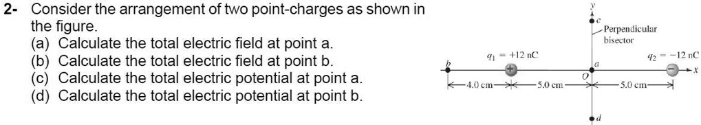
- q1=+12 nCq_1 = +12\, \text{nC}q1=+12nC located 5.0 cm to the left of point a.
- q2=−12 nCq_2 = -12\, \text{nC}q2=−12nC located 5.0 cm to the right of point a.
- Distance from point a to both charges = 5.0 cm = 0.050 m.
- Distance from point b to q1q_1q1: 4.0 cm=0.040 m4.0\, \text{cm} = 0.040\, \text{m}4.0cm=0.040m; from point b to q2q_2q2: 9.0 cm=0.090 m9.0\, \text{cm} = 0.090\, \text{m}9.0cm=0.090m.
- k=14πε0=8.99×10⁹ Nm2/C2k = \frac{1}{4\pi \varepsilon_0} = 8.99 \times 10^9 \, \text{Nm}^2/\text{C}^2k=4πε01=8.99×109Nm2/C2
(a) Total Electric Field at Point a
Electric field due to a point charge:E=k∣q∣r2E = \frac{k |q|}{r^2}E=r2k∣q∣
At point a, the electric fields due to both charges are equal in magnitude and opposite in direction.
- E1=8.99×109×12×10−9(0.05)2=43176 N/CE_1 = \frac{8.99 \times 10^9 \times 12 \times 10^{-9}}{(0.05)^2} = 43176 \, \text{N/C}E1=(0.05)28.99×109×12×10−9=43176N/C (to the right due to +q)
- E2=8.99×109×12×10−9(0.05)2=43176 N/CE_2 = \frac{8.99 \times 10^9 \times 12 \times 10^{-9}}{(0.05)^2} = 43176 \, \text{N/C}E2=(0.05)28.99×109×12×10−9=43176N/C (to the left due to -q)
Net field:Enet at a=E1−E2=0 N/CE_{\text{net at a}} = E_1 – E_2 = 0 \, \text{N/C}Enet at a=E1−E2=0N/C
✅ Answer (a): 0 N/C0 \, \text{N/C}0N/C
(b) Total Electric Field at Point b
- Distance to q1q_1q1: r=0.04 mr = 0.04\, \text{m}r=0.04m
- Distance to q2q_2q2: r=0.09 mr = 0.09\, \text{m}r=0.09m
E1=k⋅12×10−9(0.04)2=6.74×10⁴ N/C (to the left)E_1 = \frac{k \cdot 12 \times 10^{-9}}{(0.04)^2} = 6.74 \times 10^4 \, \text{N/C} \text{ (to the left)}E1=(0.04)2k⋅12×10−9=6.74×10⁴N/C (to the left)E2=k⋅12×10−9(0.09)2=1.33×10⁴ N/C (to the left; since q₂ is negative)E_2 = \frac{k \cdot 12 \times 10^{-9}}{(0.09)^2} = 1.33 \times 10^4 \, \text{N/C} \text{ (to the left; since q₂ is negative)}E2=(0.09)2k⋅12×10−9=1.33×10⁴N/C (to the left; since q₂ is negative)
Both fields point left at b, so they add:Enet at b=6.74×10⁴+1.33×104=8.07×10⁴ N/CE_{\text{net at b}} = 6.74 \times 10^4 + 1.33 \times 10^4 = 8.07 \times 10^4 \, \text{N/C}Enet at b=6.74×10⁴+1.33×104=8.07×10⁴N/C
✅ Answer (b): 8.07×10⁴ N/C, to the left8.07 \times 10^4 \, \text{N/C}, \text{ to the left}8.07×10⁴N/C, to the left
(c) Total Electric Potential at Point a
Electric potential is scalar:V=kqrV = \frac{kq}{r}V=rkqV1=8.99×109⋅12×10−90.05=2.1576×10⁴ VV_1 = \frac{8.99 \times 10^9 \cdot 12 \times 10^{-9}}{0.05} = 2.1576 \times 10^4 \, \text{V}V1=0.058.99×109⋅12×10−9=2.1576×10⁴VV2=8.99×10⁹⋅(−12×10−9)0.05=−2.1576×10⁴ VV_2 = \frac{8.99 \times 10^9 \cdot (-12 \times 10^{-9})}{0.05} = -2.1576 \times 10^4 \, \text{V}V2=0.058.99×109⋅(−12×10−9)=−2.1576×10⁴VVnet at a=V1+V2=0 VV_{\text{net at a}} = V_1 + V_2 = 0 \, \text{V}Vnet at a=V1+V2=0V
✅ Answer (c): 0 V0 \, \text{V}0V
(d) Total Electric Potential at Point b
V1=8.99×109⋅12×10−90.04=2.697×10⁴ VV_1 = \frac{8.99 \times 10^9 \cdot 12 \times 10^{-9}}{0.04} = 2.697 \times 10^4 \, \text{V}V1=0.048.99×109⋅12×10−9=2.697×10⁴VV2=8.99×10⁹⋅(−12×10−9)0.09=−1.1987×10⁴ VV_2 = \frac{8.99 \times 10^9 \cdot (-12 \times 10^{-9})}{0.09} = -1.1987 \times 10^4 \, \text{V}V2=0.098.99×109⋅(−12×10−9)=−1.1987×10⁴VVnet at b=2.697×10⁴−1.1987×104=1.4983×10⁴ VV_{\text{net at b}} = 2.697 \times 10^4 – 1.1987 \times 10^4 = 1.4983 \times 10^4 \, \text{V}Vnet at b=2.697×10⁴−1.1987×104=1.4983×10⁴V
✅ Answer (d): 1.50×10⁴ V1.50 \times 10^4 \, \text{V}1.50×10⁴V
📚 Explanation
In electrostatics, the electric field and potential are fundamental concepts describing the influence of charges on their surroundings. The electric field is a vector quantity, meaning direction matters, while electric potential is scalar, meaning only magnitude is considered.
At point a, which lies equidistant between two equal and opposite charges, the electric fields due to each charge are equal in magnitude but opposite in direction. The positive charge pushes the field away, and the negative pulls toward it — both pointing in opposite directions. Therefore, the net electric field cancels out to zero at that midpoint. Likewise, since electric potential is a scalar, and both charges have the same magnitude but opposite sign at equal distances, their potentials cancel out, yielding zero net potential.
At point b, closer to the positive charge and farther from the negative charge, both electric fields from the charges point in the same direction—toward the negative and away from the positive—resulting in a strong net field to the left. The potentials from each charge do not cancel here because the distances are unequal. The closer positive charge contributes more, but the negative charge still subtracts some potential. This leads to a positive net potential at point b.
Understanding these principles is key in fields like electronics, physics, and engineering, where managing electric forces and potentials governs device behavior.