Consider the transfer function

Here are the solutions to the problems presented in the image, including the MATLAB code and explanations.

Problem 1 Solution

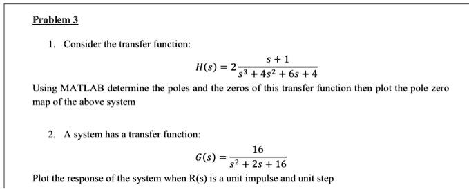
Task: Determine the poles and zeros of the transfer function H(s) and plot the pole-zero map using MATLAB.

Transfer Function:
H(s) = 2 * (s + 1) / (s³ + 4s² + 6s + 4)

Poles and Zeros:

• Zero: s = -1
• Poles: s = -2, s = -1 + j, s = -1 – j

% Problem 1: Poles, Zeros, and Pole-Zero Map for H(s)

% Define the numerator and denominator coefficients for H(s)
num_H = [2 2];       % Represents 2s + 2
den_H = [1 4 6 4];   % Represents s^3 + 4s^2 + 6s + 4

% Create the transfer function object
H = tf(num_H, den_H);

% Determine the zeros and poles
zeros_H = zero(H)
poles_H = pole(H)

% Plot the pole-zero map
figure;
pzmap(H);
title('Pole-Zero Map of H(s)');
grid on;

Problem 2 Solution

Task: Plot the unit impulse and unit step response of the system G(s).

Transfer Function:
G(s) = 16 / (s² + 2s + 16)

% Problem 2: Impulse and Step Response for G(s)

% Define the numerator and denominator coefficients for G(s)
num_G = [16];        % Represents 16
den_G = [1 2 16];    % Represents s^2 + 2s + 16

% Create the transfer function object
G = tf(num_G, den_G);

% Plot the unit impulse response
figure;
impulse(G);
title('Unit Impulse Response of G(s)');
grid on;

% Plot the unit step response
figure;
step(G);
title('Unit Step Response of G(s)');
grid on;

Explanation

For the first problem, we analyze the transfer function H(s). The zeros of a system are the roots of the numerator polynomial, and the poles are the roots of the denominator. These values determine the system’s dynamic characteristics. Using MATLAB, we define the numerator [2 2] and denominator [1 4 6 4] as coefficient vectors. The zero command finds the root of 2s + 2 = 0, giving a single zero at s = -1. The pole command solves the cubic equation in the denominator, yielding three poles: one real pole at s = -2 and a complex conjugate pair at s = -1 ± j. The pzmap function visualizes these on the complex plane, with an ‘o’ for the zero and ‘x’s for the poles. Since all poles are in the left-half plane, the system is stable.

For the second problem, we examine the time response of G(s). This system is a classic second-order system. We use MATLAB’s impulse and step functions to plot its response to a unit impulse and a unit step input, respectively. By comparing G(s) to the standard form ωn²/(s² + 2ζωn s + ωn²), we find the natural frequency ωn = 4 rad/s and the damping ratio ζ = 0.25. Since the damping ratio is between 0 and 1, the system is underdamped. This is reflected in the plots: both the impulse and step responses exhibit oscillations that decay over time. The step response rises, overshoots its final steady-state value of 1, and settles, which is characteristic behavior for an underdamped system